Copyright Notice: This article is Copyright AI Factory Ltd. Ideas and code belonging to AI Factory may only be used with the direct written permission of AI Factory Ltd.
The world is moving on from creating AI engines using prescriptive linear evaluations. Nowadays neural nets are taking over based on deep learning ideas to learn to play with no tailored algorithmic input at all. However much of AI Factory's history is based on linear evaluation. We needed to quickly upgrade our ancient Backgammon engine, so elected to create a new engine based on linear evaluation. However this offered a chance to try tuning experiments, also providing interesting insights into the properties of a tuned space, and to compare outcomes with neural-based Backgammon to see how tuned linear evaluation might compare.
This article shows what we found and how we had to adapt to tuning ideas. We were then able to compare our performance with an external neural-based Backgammon.
Background
We had already setup advanced tuning for Spades for Bandit (NTBEA) algorithm and Climber (RMHC) algorithm by Rokas Ramulionis at QMUL. However this work has stalled for a while as the fitness algorithm used for this turned out to be far too slow. We will return to this using fitness based on the system we are using here with Backgammon.
For Backgammon we chose to adopt a similar approach to the one we used to create a Poker engine for Microsoft (see "The Computer Learns to Play Poker"). This simple system worked very well for Poker.
Setting Up
The idea behind the linear evaluation for Backgammon we created was based on evaluating the apparent advantage of all possible plays for the dies given. i.e. if there was only one die left this might generate 6 or so possible legal moves but given 4 dies (an unused double, giving 4 dies) then there might easily be 100 or more possible plays. The linear evaluation then assessed various terms that considered how vulnerable the player was and also the freedom. This was mirrored for both sides. This evaluation did not need to speculatively trial different die throws as it only evaluated known existing throws for the current player.
Adapting for tuning
The evaluation was divided into the following basic terms:
| (1) | Progress | |
| This is simply a measure of how far pieces have progressed on the board. | ||
| (2) | Vulnerability | |
| This assessed the probability that a blot could be struck to the bar. It also assessed double blots that, although "safe" from being struck to the bar, were potentially vulnerable if either blot needed to move. | ||
| (3) | Blocking | |
| This assessed to what degree each piece is blocked from making progress. It provides an ordered list of blocked pieces, scoring the top block at full value with a diminishing penalty for lesser blocks. | ||
| (4) | Freedom | |
| This is in a sense the inverse of blocking above, but is equally assessed for all pieces. | ||
| (5) | Bar blocked score | |
| This assesses how blocked pieces on the bar are. | ||
| (6) | Primes assessment | |
| This assesses the extent that one side has created a wall of blocking pairs or greater that the opponent either cannot, or has limited chances, to pass. |
The above algorithm is a conventional type of design for a hand-crafted prescriptive linear algorithm. Choice of parameters can be hand-crafted to adopt reasonable rule-of-thumb values. Every part of this was an explicit encoding of a specific heuristic idea.
This can then be setup to allow automatic tuning, by introducing a macro "K" that can either point to a constant array, or an array of values during tuning, as follows:
progress_score+=(prog*playerBoard[i]*K(1));
Here K(1) is the variable that may either point to a constant or variable array.
This whole approach is predicated entirely on values estimated to directly contribute to the move choice. However this structure could easily not map to a good solution, even with optimised parameters. The algorithm needs to add open parameters that are not based on any rule-of-thumb heuristic idea but that allow modification of the eventual value to a better solution. e.g.
| progress_score += progress_score*K(23)/(50+movenum); | |
| progress_score -= progress_score*K(24)/(150-movelim); |
Here the value of the parameter is scaled by the move number "movenum". "movelim" above is the same as movenum, but limited to a maximum value of 100. These two parameters K(23) and K(24) provide a varying modification of the progress score, depending on the move number in the game.
As it happens the actual values in the tuned engine in this case are K(23)=0 and K(24)=8. This gives the following profile:
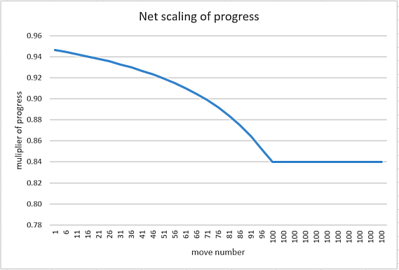
Figure 1: Progress score scaling linked to move number
However with K(23)=50 and K(24)=4 it would have provided a magnifier (that could still be scaled by the earlier K(1))
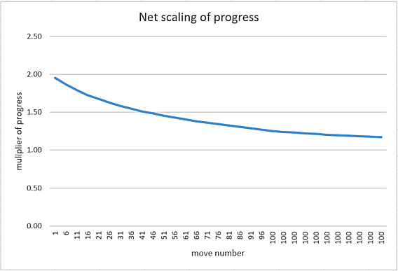
Figure 2: An alternative scaling
This is repeated on all 6 heuristic terms listed earlier, needing a total of 12x K parameters. In addition a similar formula is applied for scaling all these for before and after auto bear off is possible.
The addition of these 12 extra terms substantially improved the performance of the program.
In total the linear evaluation has 73 parameters.
What is the basis for Tuning?
How do we tune? A candidate would be to trial a parameter set in a trial of games against the base version. This is essentially how our Spades tests worked. The Backgammon engine is much faster than our Spades but I estimated that this would likely be too slow. So we setup a very different arrangement as follows:
| (a) | We created a set of 100 games played at a very high play level. | |
| (b) | We then analysed each game by running multiple Monte Carlo trials for each move in that game counting how often each move resulted in a win. This took about 2 days per game (run on a 32-core Threadripper) | |
| (c) | To test a new parameter change, it compared the top play choice with the current parameter set with every move in all 100 games, counting how often this lead to a win. This was tweaked to not just being sum(win counts) but sum(relative win counts), where each win count was weighted as "win count" - "worst win count for this position". So if the new parameters picked the least successful move it would earn zero points for that move. If most moves had similar win counts then all moves would earn similar small credits. This stops the tuning applying high values where most moves yield similar chances of wins. Where the top move is much better then the credit value is very high. |
The table for "b" above for a single game would look like the sample table below. The index position of the counts below corresponded to the moves in the legal moves list, so therefore the line "1" below had 7 legal moves. Die throw moves were marked by just "-1".
| TInt DATA01_anal[KMaxMovesInGame][KMaxPossibleTurnsLimited] = { // 0EL | |||||
| /* | 1 */ { | 3209, 2791, 2613, 3262, 2964, 3008, 2928, -1 }, | |||
| /* | 2 */ { | 3125, 2901, 4450, 3292, 3361, -1 }, | |||
| /* | 3 */ { | -1 }, | |||
| /* | 4 */ { | 2325, 2291, 2383, 3126, 2044, 2133, 2707, -1 }, | |||
| /* | 5 */ { | 2839, 2161, 4259, 2892, -1 }, | |||
| /* | 6 */ { | -1 }, | |||
| /* | 7 */ { | 3120, 2858, 3063, 3825, 4394, -1 }, | |||
| /* | 8 */ { | 3683, 4841, 5764, -1 }, | |||
| /* | 9 */ { | -1 }, | |||
| /* | 10 */ { | 3536, 4099, 3159, 3626, 2948, -1 }, | |||
| /* | 11 */ { | 3253, 3703, 2746, 2334, 3384, 2516, -1 }, | |||
| } | |||||
The procedure to tune was to initially randomly change a subset of the 73 parameters, looking for a set that scored higher. That was then made the new base set and the process repeated. This finally provided a new set of parameters that could be tested in actual play. The selection of which parameters to modify was randomly selected and number to actually change also randomly selected (See Fig. 3 below, which shows the parameter tested, followed by relative change in brackets). The tuning of any one set continued until no further improvements could be found.
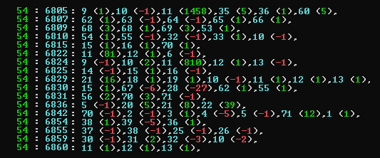
Figure 3: A list of parameters tried (blue) with the bracketed offset from original value
Our generic framework is comfortably set up to allow easy tournament testing so that any new variant of the parameter set could easily be tested against multiple versions. In practice we tested 7 new sets in a round-robin against all other tested versions and against the current established best version. An example tournament test result looked like this (Figure 4):
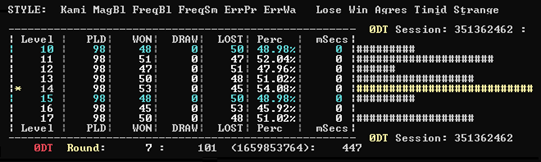
Figure 4: A tournament table
Here the tournament has only been run for 98 played games for each version (normally this might run for some 150k games). From this the current best performer is highlighted in yellow with a 54.08% win rate. In this table the reference level is level 10 and levels 11 to 17 each represent another unique new set of tuned parameters, each of which is a tuned optimum set. In this case set 14 is winning overall, but is not significant as very few rounds have actually been run. This arrangement of a round robin of multiple candidate new versions against a base known best is much better than a simple head-to-head as it proves each against a variety of possible opponents, so that it does not deliver a "new best" just based on a quirk that arises between just 2 levels.
Running the tests
Choosing from all parameters to tweak at random could easily to be too wide a cast, so tuning runs were each time assigned a particular subset of the parameters to tune, as follows:
| const TInt KLearn_Set1[] = { // all imaginable | |||
| 1,2,3,4,5,6,7,8,9,10,11,12,13,14,15,16,17,18,19,20,21,22,23,24,25,26,27,28,29,30, | |||
| 31,32,33,34,35,36,37,38,39,40,41,42,43,44,45,46,47,48,49,50,51,52,53,54,55,56,57,58,59,60, | |||
| 61,62,63,64,65,66,67,68,69,70,71,72,73,0 | |||
| }; | |||
| const TInt KLearn_Set2[] = { // tuning just vulnerability | |||
| 3,4,5,6,7, 22, 25,26, 38, 65, 72,73,0}; | |||
| }; | |||
This allows a more thorough exploration of a limited set of related parameters. In practice these runs tended to reach some terminal point quite quickly after perhaps 15 to 30 minutes runtime. It will have made some 50 changes or so after some 10000 attempts to change parameters.
Tuning was further enhanced by allowing a parameter swap where the net score had not changed. This allowed sideways shifts to new equal starting positions from where it could re-randomise and detect a new best value. As a further optimisation, improvements from increasing a particular parameter would be more likely increased again, instead of a trial decrease in any further randomised change.
Peering inside the black box, dissecting what tuning actually did
This tuning procedure is evidently a black box, where a handle is cranked and new values drop out the other end. In operating it we could imagine what the characteristics of these changes might be. We had a chance to peer a little into this black box … but the behaviour did not match our expectation!

First, the process we are looking at here is evidently evaluation hill-climbing. Mentally this is an intuitive idea that our imagination maps to a 3D hill where the top of the hill is the optimum value. However that represents an evaluation with just 2 terms, X and Z, with the Y-axis being the vertical evaluation term. What we have though are 73 parameters, representing a potentially hugely 73-D complex multi-dimensional space. There is no reasonable way to provide a mental visualisation of this, so here we will have to represent this with just the 2-term evaluation and simply extrapolate our understanding from this.
First we can anticipate the impact of our initial manual tuning, seeded by rule-of thumb values. The expectation is that the initial position within the evaluation hill will clearly not be horrible. This will probably drop us in a moderate position in the evaluation landscape, shown by the red flag below
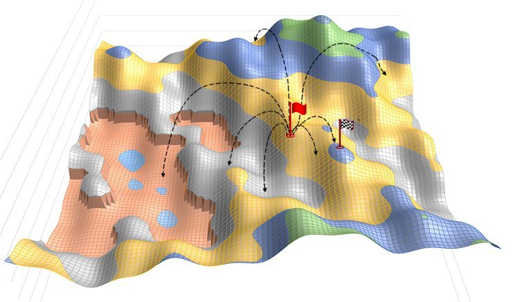
Figure 5: The first jumps to higher value, where X and Z are 2 parameters
and Y is the evaluation
From that position vast numbers of jumps are made to new random positions in the evaluation map. From these a new position is found that improves the evaluation value, shown above (Figure 5) by the checkered flag. This not an end point but the start of a series of further optimisations.
Note in our 2-parameter metaphor in Figure 5 that we have regions with tall cliffs shown on the bottom left. These emulate the idea of sudden evaluation changes in response to small parameter changes. In a hill climb procedure these might become tuning barriers that incremental parameter changes cannot cross. However a large tested tuning step might be able to jump over such a chasm and continue on the other side. This requires maintaining tuning flexibility.
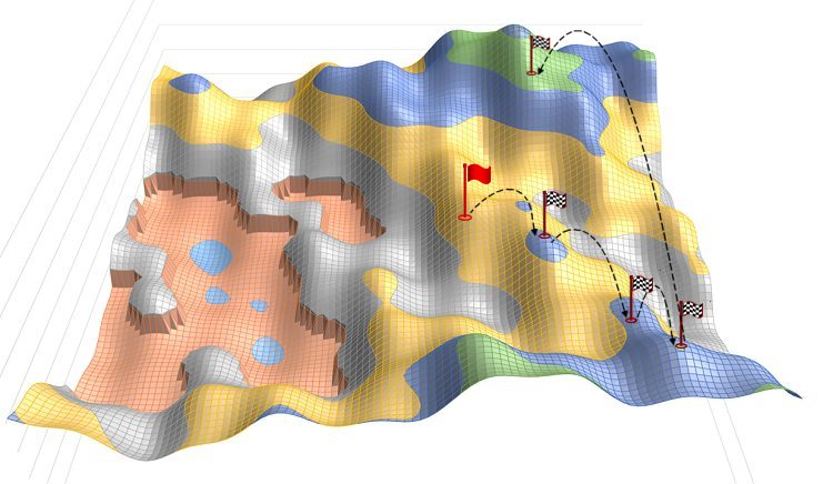
Figure 6: Multiple jumps showing a progression of increased values for the evaluation
From this first improved position the randomisation continues to jump to new optimised positions. The figure 6 above shows 4 hops, one of which jumps over a number of lower positions. The randomised jumps are not just places within close proximity of the base position, as any one random change might be large, skipping many much lower positions. It is therefore not a simple incremental hill climb, but a jumping place from where to reach new positions.
Note that as trials are run, if no further improvements are found, the trial will attempt a variety of regimes of parameter changing, switching between these. Some will require just one or even many parameter changes. Some by large and some by small increments. This maximises the chance that it will be able to continue to make progress.
Failed expectation #1- The optimisation sequences suddenly stop
The first non-intuitive outcome is that in testing there may be many jumps, say 10 to 50, but that these will stop. It seems imaginable that having reached some optimum point that further points would eventually arise, even if rare. Our regime for random changes adapts in the face of failure to provide a new best value. Of course at this point our 2-D visualisation of the 73-D space offers a rather limited inadequate emulation. To rationalise for it stopping you have to account for the fact that a number of parameters may have been changed at once. Change of a single parameter is relatively infrequent and to return to the position where many changes were being made also needs a reversed value change that drops close to that previous point with a higher evaluation value. That may be rare enough that it never occurs. The current new end point may have a significantly improved value and other higher jump off points may be very rare. This last jump, in a sense, appears to resemble a kind of narrow chink or wormhole that we have jumped through, but where jumping back is essentially impossible.
Of course a possible explanation for this might be that the evaluation delivers an unexpected incorrect high value that prohibits progress. This would easily explain the stall, but this did not happen.
Another explanation might be that the number of game samples of 100 is not enough, giving just 10,000 or so moves to test. This may leave the evaluation unable to detect small rare improvements that would allow progress to better evaluation points.
From this position we might also rationalise that we have indeed found the optimum point. However if we compare the tuned parameter set with the 6 others run in parallel, we find a further problem.
Failed expectation #2- The multiple optimisation sets do not share a common convergence
Having delivered an optimised set we might reasonably assume that the 6 other optimised 73 parameter sets will be to some degree similar. In our 2-D figure emulation figure this might manifest as a number on endpoints in some reasonable proximity of each other. These might, in the metaphor, be a number of hillocks in the vicinity of the optimum peak. It would manifest as most parameters appearing to generally shift in similar directions.
However if we examine the shifts for each parameter, we find no apparent common pattern. Each optimum parameter has seemed to have taken a completely different random choice in direction. In Figure 7 below we have the 73 parameters sorted by the number of times the value increased minus the number of times decreased. A 0/0 value indicates that the parameter never changes in any of the 7 tuned sets. If 7/0 this indicates that it increased in every set and 0/7 that it decreased in every set.
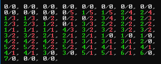
Figure 7: Sorted parameter list showing count of increased and decreased value
So each optimised parameter set has found a stable endpoint that is some distance in the 73-D space from any other optimised set. In only one instance did a parameter shift in just one direction for all 7 sets. This was not expected.
What is going on? What is the explanation?
This will review some possible conclusions:
| (1) | The tuning is poor or just broken! | |
| That would be unfortunate! However the tuned system does appear to perform well in testing, improving the program. The end product play is good, so we do not have to throw up our hands just yet. | ||
| (2) | The evaluation space is too difficult to explore. | |
| We are only offered the 2 parameter 3-D model to try and imagine this, but our 73-D evaluation space is perhaps too complex to reliably explore and true optimum points may be very hard or impossible to reach using this exploration method. Of course our methodology is quite simple and it would be rational to imagine that exploring a 73-D space offers plenty of chances of simply getting lost. Our underlying premise that we are faced generally with hill-like inclines to follow may be an inaccurate over-simplification of the evaluation space. | ||
| (3) | We should have used the Bandit (NTBEA) algorithm and Climber (RMHC) algorithm | |
| This might be true. However the above are designed to provide more optimum paths to the same type of outcome we had. However our tuning runs were fast and failed to improve given a whole day over the 10 to 30 minutes they appeared to need. However the jury is out and we may well try some experiments with the above in the future. | ||
| (4) | Evaluation terms simply overlap allowing multiple equivalent viable sets. | |
| This is a happier and rational conclusion. The various evaluation terms offer overlap in assessment. i.e. advancement high values will also offer reduced vulnerability as an advanced piece will be offered less exposure to being hit. Therefore shifting the evaluation shape of each term will offer different possible overlaps. If one term vacates some coverage of an evaluation then another term may be modified to compensate. |
How well did the tuned version perform?
We started with our original backgammon, written over 20 years ago. The first version of the new program was completed inside a few weeks with just 39 parameters and already scored 52.48% against the old Backgammon. After addition of more parameters and tuning runs the win percentage reached 56.44%. In parallel with this (to create reference strong games) it was mixed with a Monte Carlo variant, simply using the new evaluation to play out the entire game and count the win/loss count for each root move. This achieved a 68.45% against the old Backgammon, but was not a practical version though as it might take up to 10 minutes for just one move, so was used to create "perfect" reference games.
This indicates that our program was "improved" but this gives no indication of its performance against other Backgammon programs. However our colleague Chris Whittington had created a neural-based Backgammon program that was believed to play well. To test this he played it against the public domain Backgammon program created at Berkeley, University of California (https://github.com/weiss/original-bsd/blob/master/games/backgammon/common_source/backgammon.c). His program beat that program at expert level 70% of the time. This offered a point of reference for us so we took the source and interfaced it with our program. Our testing showed that we beat the Berkeley program 70.20% of the time, essentially the same result. The old Backgammon beat the Berkeley program 57.07% of the time.
Conclusion
The conclusion is that our old Backgammon was perhaps better than we thought, although it did suffer some obvious weak plays. However, by proxy of a common opponent, the new version clearly performed at about the same level as a neural-based Backgammon that was expected to play well, which was a good enough step-up to justify its use in release. However this did not just replace our old program with its 5 levels, but simply added 2 new higher levels. The reason for this is that people get into the habit of liking the version they play and simply replacing it might make many users unhappy. It is better to provide additional levels that also give them access to the enhanced version.
A significant evolution in this work is the way we create linear evaluation. This has added open terms that allow tuning to shape the evaluation, but without any directed heuristic idea attached, to simply widen the possible scope of evaluation and allow tuning to construct evaluation terms that contribute to play. This is a change in mind set that otherwise was entirely driven by clear heuristic ideas to contribute to evaluation. It is a step towards the driving mechanism of neural nets that essentially create evaluation terms entirely from simple un-directed input components.
We note though the improved performance of the Monte Carlo version. This shows that more can be achieved. However that will await a future version.
Jeff Rollason - July 2021